Bulk Arps Curve Fitting on GPU


This article proposes a method for significantly faster Arps decline curve fitting on large datasets using TensorFlow on GPUs. It tackles the limitations of traditional approaches, which rely on iterative curve fitting, like SciPy's curve_fit, applied to each data point one at a time. By leveraging TensorFlow's parallel processing and vectorization capabilities on GPUs, this method can fit multiple Arps decline curves simultaneously, achieving substantial speed improvements for large datasets.
Arps decline curve analysis (DCA) is a vital tool in the oil and gas industry for representing and predicting the future production of wells. Developed by J.J. Arps in 1945, it analyzes historical production data relying on the observation that oil and gas production typically follows a declining trend over time as the reservoir pressure depletes. By fitting the data to parametric equations, engineers can forecast how oil and gas flow will decline over time. This information is crucial for tasks like estimating reserves, planning production strategies, and making investment decisions. Essentially, Arps DCA helps maximize efficiency and profitability by providing a roadmap for oil and gas well behavior.
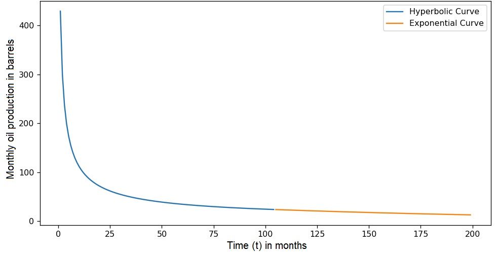
Arps divides the well production life into mainly two partitions:
- A hyperbolic curve representing the segment that starts after peak production, this is the initial stage of production characterized by a rapid decline in production rate.
- An exponential curve representing the later stage of production where the decline rate becomes more gradual and approaches a constant value over time.
The curve function is summarized as follows:
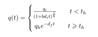
where
- q(t) is the production rate in the form of production per unit time
- t is time
- qi is the initial production
- di is the initial decline in the hyperbolic part of the equation
- b is the hyperbolic factor controlling the rate of change of the decline
After reaching a certain decline rate df (usually 7% secant decline) at time th, the curve is represented by an exponential function using qh until end of production.
As seen in Code Snippet 1, SciPy's curve_fit is usually used by defining the Arps decline function arps_production, the production time period xdata, and the production values ydata. Based on domain knowledge or engineering estimates, the fitting can be sped up by providing adequate initial values for the parameters p0, and the output can be constrained by adding the boundaries for each parameter bounds.
params, params_covariance = optimize.curve_fit(arps_production,
xdata=np.arange(len(actual_production)),
ydata=actual_production,
p0=[initial_qi, initial_di,initial_b],
bounds=([0,DF_PERCENT_SEC,B_FACTOR_LOWER_BOUND],[np.inf,SECANT_DI_UPPER_BOUND,B_FACTOR_UPPER_BOUND]))SciPy's curve_fit employs a least squares minimization algorithm. This technique iteratively adjusts the parameters of the Arps equation to minimize the sum of squared residuals between the predicted and actual production rates (ydata). Residuals represent the difference between these values. In each iteration, the algorithm calculates the gradient of the cost function (sum of squared residuals) with respect to each parameter and uses this information to update the parameters in the direction that leads to a better fit, ultimately minimizing the overall difference between predicted and observed production rates.
Conventional curve fitting algorithms, like SciPy's curve_fit, struggle with large datasets. These methods typically fit each data point individually using a separate optimization instance, making them computationally expensive for massive datasets. Additionally, SciPy's curve_fit relies on few optimization algorithms in its base package (Trust Region Reflective, dogleg and Levenberg-Marquardt's least squares minimization algorithms), which might not always be the best choice for complex models or large data volumes.
This article introduces a TensorFlow-based approach to accelerate Arps decline curve fitting by leveraging its distributed computing, complex optimization algorithms and vectorization. Here's the workflow:
- Load production data for all wells containing time t and monthly production rates q into two Tensors.
- Define the Arps decline curve equation within a TensorFlow function.
- This function will take time t as input and utilize initial production rate qi, initial decline di, and B-factor b as variables.
- The function outputs the predicted production rate based on the chosen model parameters.
- Define a loss function that calculates the difference between the predicted production rate from the model and the actual production rate q.
- Common loss choices include mean squared error (MSE) or mean absolute error (MAE).
def loss():return tf.reduce_mean(tf.square(arps_production_tf_vectorized(t,[qi, di, b]) - q))- Utilize a TensorFlow optimizer (e.g., Nadam optimizer) to minimize the loss function across all data points simultaneously over (n) epochs.
optimizer = tf.keras.optimizers.Nadam(learning_rate=LEARNING_RATE, beta_1=BETA_1, beta_2=BETA_1)- Define the constraints for each of the model parameters.
- This single optimization step fits a different Arps decline curve to each data point in the entire dataset.
for _ in range(NUMBER_OF_EPOCHS):  # number of optimization steps
	optimizer.minimize(loss, params) # add constraints
	qi.assign(tf.clip_by_value(qi, clip_value_min=0, 	clip_value_max=float('inf')))
	di.assign(tf.clip_by_value(di, clip_value_min=DF_PERCENT_SEC_T,
	clip_value_max=SECANT_DI_UPPER_BOUND_T))
    b.assign(tf.clip_by_value(b,
clip_value_min=B_FACTOR_LOWER_BOUND, clip_value_max=B_FACTOR_UPPER_BOUND))- Evaluate the fitted model performance using metrics like Mean Absolute Percentage Error (MAPE) or Mean Absolute Error (MAE).
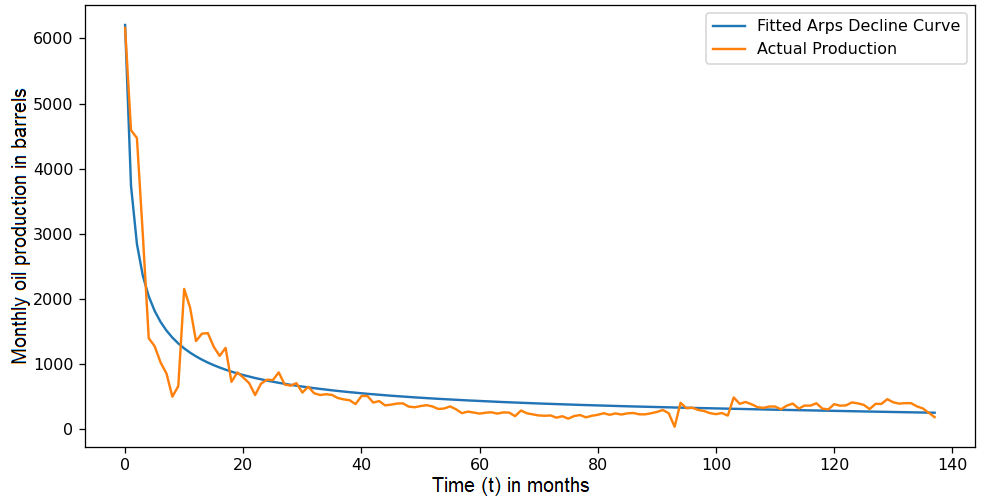
- Visualize the fitted curve compared to the actual production data for validation.
The core strength of TensorFlow lies in two key features. The first is its vectorized distributed computing architecture. Unlike SciPy's curve_fit which is confined to a single CPU core, TensorFlow efficiently distributes the workload across the multiple GPUs available in your system, fitting the Arps decline equation to millions of data points simultaneously. The second is its wider range of optimization functions, while SciPy's curve_fit often relies on few optimization algorithm in its base package, which might not always find the absolute best solution, especially with massive datasets and potential complexities. TensorFlow offers a vast arsenal of optimization algorithms (Adam, Nadam, SGD, etc.). Even though SciPy provides a broader optimization library (scipy.optimize which adds a few extra optimizers like Nelder-Mead simplex algorithm and Differential Evolution), utilizing these alternatives requires manual implementation of the optimization loop.
A crucial aspect of this approach is evaluating its effectiveness against traditional curve fitting methods. Our investigation focused on two key areas: fitting error and time performance. Interestingly, both approaches yielded comparable fitting errors (SciPy's curve_fit scored an average MAPE of 0.65% across all datasets, while the Tensorflow method scored an average MAPE of 0.67%), indicating that the TensorFlow method accurately replicates the curve fitting behavior of SciPy's curve_fit. However, the true advantage lies in time performance.
To achieve a fair comparison, we employed two machines from Azure with similar budgets. The first machine, a GPU-based system (2 V100 GPUs, 32 GiBs GPU memory, and 224 GiBs RAM ), served as the platform for the TensorFlow approach using the Nadam optimizer. The second machine, a CPU-based system (72 vCPUs, and 144 GiBs RAM ), ran the traditional method using the Trust Region Reflective algorithm's least squares minimization and code based parallelization where each core was responsible for fitting a chunk of the dataset. Our findings revealed that the TensorFlow method on the GPU significantly outperformed the CPU-based approach with larger datasets. This performance improvement becomes more pronounced as the dataset size increases, making the TensorFlow method ideal for large-scale production analysis.
This plot shows the improvement in performance over different dataset sizes for the two machines (NC12s v3 VS F72s v2):
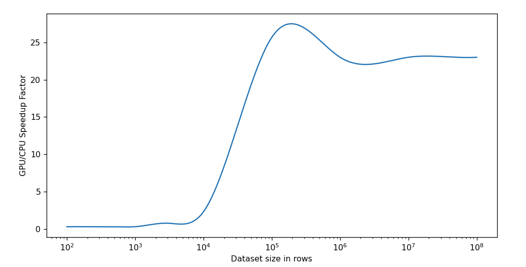
Due to the overhead incurred by TensorFlow's initialization, there isn't a noticeable improvement compared to the CPU-based method for smaller datasets. However, as the dataset grows larger, the improvement over the CPU method exponentially increases. Once the dataset becomes larger than the GPU's memory, the improvement factor slightly decreases as a new overhead is introduced when the dataset has to be broken down into chunks based on the GPU memory limit. The improvement factor then plateaus since TenforFlow now must process the chunks sequentially. We can further increase the improvement factor and delay the plateau by increasing the number of GPUs or using GPUs with more memory.
Conclusion
TensorFlow offers a compelling approach to Arps decline curve fitting, particularly for large datasets. It leverages GPU parallelization and vectorization to deliver significant speedups compared to traditional techniques. This enhanced efficiency scales well as data size increases, making it ideal for real-world scenarios. Additionally, TensorFlow provides flexibility in customizing the Arps decline model, loss function, and optimizer, enabling tailored analysis to address specific needs. This empowers engineers to analyze larger datasets faster, leading to quicker production forecasting and optimized reservoir management decisions.
References
- Arps, J. J. (1945). Analysis of decline curves. Transactions of the AIME, 160(1), 228-247.
- SciPy curve_fit: https://docs.scipy.org/doc/scipy/reference/generated/scipy.optimize.curve_fit.html
- https://www.tensorflow.org/
- Microsoft. (2023, March 28). Azure Virtual Machines. https://learn.microsoft.com/en-us/azure/virtual-machines/