Inductive Clustering For Lower Dimension Input Vectors


Introduction
We often need to expand or generalize the output of clustering algorithms for unseen data points in training without recomputing the clustering. Some clustering algorithms support this by nature, which is called Inductive Clustering. This article will discuss extending the non-inductive clustering algorithms to classify new instances and classify data samples with lower dimensions than those used for creating clusters.
Keywords: Inductive Clustering, Clustering Generalization
Problem Definition
Let us start by introducing some concepts from the oil and gas industry.
- Completion Features: features that describe the process of making a well ready for production after drilling operations
- Proved Developed Producing Oil and Gas Reserves (PDPs): oil and gas wells that are proven to have a production and already producing
- Proven Undeveloped Oil and Gas Reserves (PUDs): oil and gas Reserves that are proven to have oil production but still some development and execution are remaining before the oil is produced.
Some Context
In Rasia, we use a mix of learning and rule-based algorithms for clustering PDPs. These clusters are made from the wells' location, and geological features. We can then use these clusters to verify the production prediction for a given well by comparing it to other wells within its cluster.
Goal
We aim to generalize these clusters for PUDs to predict the production and completion feature patterns for a given PUD by assigning the PUD to one (or more) of the existing clusters. To achieve this, we will need to tackle the following challenges:
- For PUDs, we do not have as many features as we do for PDPs.
- Try not to modify the clustering scheme as much as possible.
- Try to assign multiple clusters for each well with a given probability for each cluster to capture the difference between the dimensions of PUDs and PDPs
We can formulate this by repreasenting a PUD feature vector \( x \in R^{n-m} \) and set of the cluster \( \{ c_1, c_2, ..., c_k \} \) that is generated from PDPs feature vectors \( v \in R^{n} \).
Our goal is to assign a probability for each cluster \( \{ p_1, p_2, ..., p_k \} \) that represents how likely this PUD will be in this cluster after completion.
Inductive Clustering Algorithms
Some clustering algorithms induce functions for classifying the whole space of interest; these methods are called inductive clustering. An example of these algorithms is the fuzzy c-means clustering algorithm. Instead of putting each data point into separate clusters, a probability of that point being in that cluster is assigned. In fuzzy clustering, also called soft clustering, each data point can belong to multiple clusters along with its probability score or likelihood.
In our problem, using any of the soft clustering algorithms will have two main downsides: firstly, it will require a complete change in our clustering scheme. Secondly, it will only work if the test data sample has the same features as the training data or \( R^{n-m} = R^{n}\) .
Extending Clustering With Estimators
Instead of changing the clustering scheme, we can use the clustering output to train an inductive model with a classifier and use this classifier to scale to new data. This approach has several benefits:
- It works independently from the used clustering algorithm, which makes this a modular approach that is consistent over time.
- It allows us to use the inferential characters of the classifier to describe or explain the clusters, more on this later.
Another essential benefit for our use case is that we can train the classifier using only the location features to use the model for PUDs.
Choosing the classifier
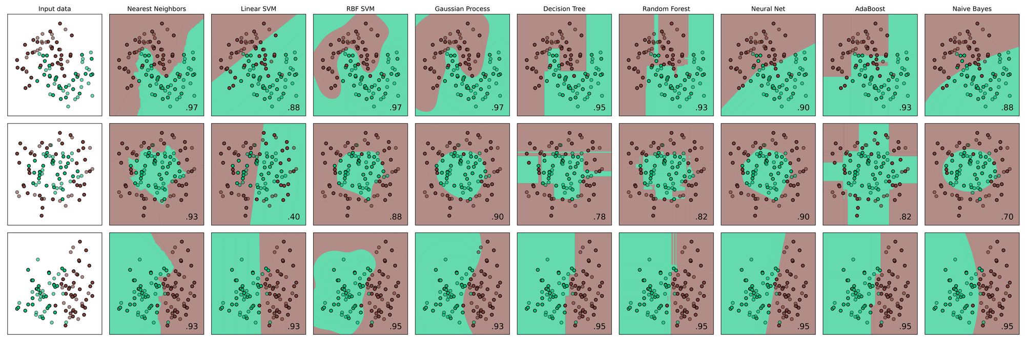
The choice of the classification algorithm will influence the properties of generated clustering regions. As we cannot determine how the clustering regions will fill all the input space from the input data, a proper understanding of both the decision boundaries generated from different algorithms and the nature of the problem you are trying to solve are essential for choosing the best algorithm for the problem.
Implementation Walkthrough
Looking at the data
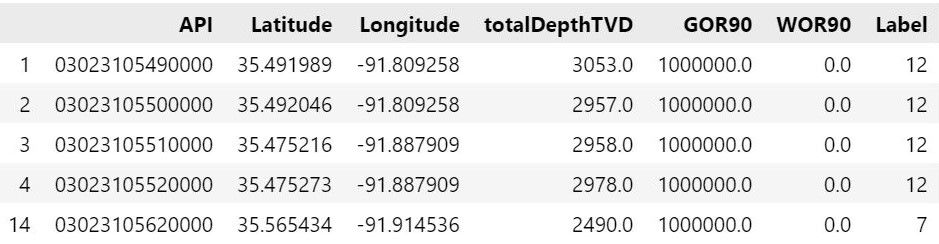
This dataframe contains the PDP data that is used for generating clusters, and the output cluster for each well, the description of each feature is as follows:
- API: Id for each well
- Latitude: location information for well
- Longitude: location information for well
- totalDepthTVD: total true vertical depth
- GOR90: gas to oil ratio (geological feature)
- WOR90: water to oil ratio (geological feature)
- Label: Id for the cluster to which the well belongs
As we mentioned earlier, we will only use Latitude and Longitude features to train our model as they are the only available features for PUDs case.
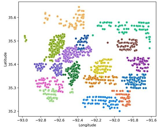
Plotting clusters with location features
Before training our classifier, we need to know the amount of lost information by using only the location features. We can discern it by showing the overlap between clusters when projected onto the lat-long 2D plane.
Classifier Training
We will start our experiments by training a KNN classifier using Longitude and Latitude as the features and see our performance on the validation set. We use RobustScaler from sklearn for features scaling to minimize the effect of outliers and make_pipeline to combine features preprocessing, and model in one interface.
X = df[["Longitude", "Latitude"]].values
y = df['Label'].values

X_train, X_test, y_train, y_test = train_test_split(X, y, test_size=0.33, random_state=42)

knn = KNeighborsClassifier()

knn_pipe = make_pipeline(RobustScaler(), clf)
knn_pipe.fit(X_train, y_train)
print(f"Validation Accuracy: round({knn_pipe.score(X_test, y_test)}, 3)")
>>>>> Validation Accuracy: 0.987Top-3 Accuracy Improvement
Instead of predicting one cluster, we can use the predict_proba function to predict a probability for every cluster, these probabilities can be used to determine if the well is in an area with overlapping clusters.
from sklearn.metrics import top_k_accuracy_score
y_hat = pipe.predict_proba(X_test)
print(f"Validation top-3 Accuracy: {top_k_accuracy_score(y_test, y_hat, k=3)}")
>>>>> Validation top-3 Accuracy: 1.0
Comparing The Clustering Regions From KNN and RF
To compare clustering boundaries from KNN and RF models. We will train an RF model the same as we did for KNN, then use the model to predict all the points in the space and plot the outputs.
rf = RandomForestRegressor(n_estimators=10)
rf_pipe = make_pipeline(RobustScaler(), clf)
rf_pipe.fit(X_train, y_train)To create an input representing all input space, we need to create a grid with a specific resolution using min and max values for Longitude and Latitude the pass this grid as input to the two models.
x0_min, x0_max = df["Longitude"].min(), df["Longitude"].max()
x1_min, x1_max = df["Latitude"].min(), df["Latitude"].max()

xx0, xx1 = np.meshgrid(
np.linspace(x0_min, x0_max, 800),
np.linspace(x1_min, x1_max, 800),
)

X_grid = np.c_[xx0.ravel(), xx1.ravel()]
knn_response = knn_pipe.predict(X_grid)
rf_response = rf_pipe.predict(X_grid)
Plotting the resulted boundaries using contourf function from matplotlip
fig, axs = plt.subplots(1, 2)
fig.set_size_inches((14, 6))

axs[0].contourf(xx0, xx1, rf_response, levels=len(data["Label"].unique()), alpha=0.6)
axs[0].set_title('Random Forest')

axs[1].contourf(xx0, xx1, knn_response, levels=len(data["Label"].unique()), alpha=0.6)
axs[1].set_title('knn')

for ax in fig.get_axes():
    ax.label_outer()

plt.show()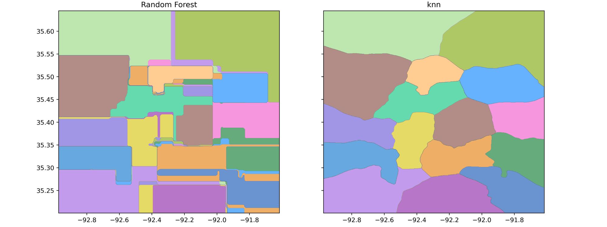
Comparing the two outputs, we found that the regions created from the KNN model are more suitable for our use case as they are more understandable and can be visualized easily with maps applications.
Conclusion
In this article, we discussed the concept of inductive and non-inductive clustering and how to extend non-inductive algorithms for classification over all input space. We also discussed handling cases when we need to cluster data with dimensions lower than the data used for creating clusters and how this can be useful for solving a real business problem.
References
- Miyamoto, Sadaaki. (2012). Inductive and non-inductive methods of clustering. Proceedings - 2012 IEEE International Conference on Granular Computing, GrC 2012. 12-17. 10.1109/GrC.2012.6468710.
- James C. Bezdek, Robert Ehrlich, William Full, FCM: The fuzzy c-means clustering algorithm, Computers & Geosciences, Volume 10, Issues 2–3, 1984, Pages 191-203, ISSN 0098-3004, https://doi.org/10.1016/0098-3004(84)90020-7.
- Inductive Clustering sklearn documentation: https://scikitlearn.org/stable/auto_examples/cluster/plot_inductive_clustering.html