Raisa's Domain and Time Series Prediction

• One of the things we do at Raisa is forecasting oil and gas production for all wells in the United States. Forecasting are usually done for the next twelve months based on previous data, which is by definition a time series forecasting problem.
• With the rise of transformers in Natural Language Processing and Computer Vision, we conducted an experiment that tries to use transformers to predict the data described above.
• This blog summarizes one of many experiments which is Ordinal Regression (Classification)

Motivation

• Why did we choose Ordinal Regression instead of Regression?
• We tried to use regression at first but the results were not impressive, which pushed us to try and re-examine the way we look at our data and our problem.
• Since transformers are already proven as Language Models, we thought that we could create a "Well Model".  
• Just like you could give a Language Model a prompt and it would continue and come up with a full sentence, We wanted to train a "Well Model" that you could give some production values and it would predict the rest of the production stream as if it was predicting words to complete a sentence.

Data Processing

• To apply classification on continuous data, we needed to bin the data so that we can treat each production value similar to a word in a corpus

Binning Algorithm

• The algorithm we used for binning was quantile binning but with a slight modification.

Quantile binning: Values are binned so that each bin contains a certain percentage of values.

• The modification we added is that instead of moving to a new bin after reaching a certain percentage of the data, we added a threshold for the difference between each bin and the next one.
• If we have an array of bins \( B = b_1, b_2, ..., b_n \), this rule applies to almost all of the bins \( b_{i+ 1} - b_{i} < 0.1 * b_{i} \)
• We applied this rule after the value of 100 barrels, as before then 10% of a value would be very negligible.
  • e.g. 10% of 2 is 0.2, which would mean that the value 2 would be its own bin no matter what percentage of values is in it.
• This was done to reduce the information lost when binning the production values while making sure each bin has enough data in it for the training process

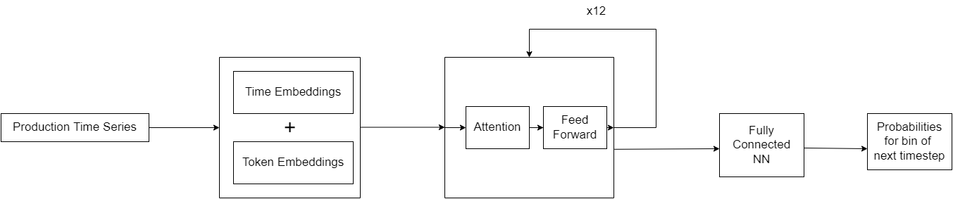
Model Architecture

• As we wanted to have a model that can generate new timesteps given some production values, we thought a decoder architecture would be the most fitting and chose the GPT2 to be the body of the model.

• We will show how we implemented this using PyTorch

Data Embeddings

• The first step in our model was how to transform the bins into vectors and add the time encodings, for that we chose a simple nn.Embedding layer for both time and token embeddings

class DataEmbeddings(nn.Module):
    def __init__(self, config: DecoderConfig):
        self.config = config
        self.time_positional_encoding = nn.Embedding(MAX_TIMESTEPS, config.embed_dim)
        self.token_embedding = nn.Embedding(config.num_of_bins, config.embed_dim)

    def forward(self, x: torch.Tensor, pos: torch.Tensor):
        token_embedding = self.token_embedding(x)
        time_embedding = self.time_positional_encoding(pos)

        return token_embedding + time_embedding

Decoder

• The decoder consists of many different parts that we need to define before creating the decoder itself, those things include DecoderBlock, FeedForward, and MultiHeadSelfAttention.

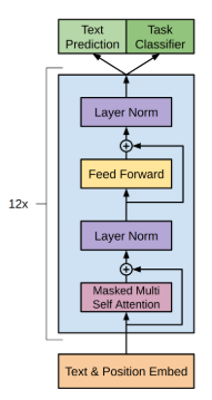
Retrieved from https://amaarora.github.io/2020/02/18/annotatedGPT2.html

Attention

• To simplify attention as much as possible, think of it as a weighted average of the features given to the transformer, where the weights are learned during training.

class AttentionHead(nn.Module):
    def __init__(self, config: DecoderConfig, attention_head_dim: int) -> None:
        super().__init__()
        self.q = nn.Linear(config.embed_dim, attention_head_dim)
        self.k = nn.Linear(config.embed_dim, attention_head_dim)
        self.v = nn.Linear(config.embed_dim, attention_head_dim)

    def forward(self, x, causal_mask, padding_mask):

        return scaled_dot_product_attention(self.q(x), self.k(x), self.v(x), causal_mask, padding_mask)

• The function scaled_dot_product_attention is the averaging step, you will notice that we pass the tensor x to the function as the key, value, and query which is why we call it self-attention.
• You will notice that the function takes causal_mask and padding_mask as arguments, these are used to ignore certain timesteps during the attention.

def safe_softmax(x, eps=1e-8):
    """Softmax modified so that we can output 0 in all elements
    i.e. pay attention to 0 timesteps"""
    e_x = torch.exp(x - x.max())
    return e_x / (e_x.sum(dim=-1, keepdim=True) + eps)


def scaled_dot_product_attention(q, k, v, causal_mask, padding_mask):

    scores = torch.bmm(q, k.transpose(1, 2)) / math.sqrt(q.size(-1))

    # If element is True, then we don't want to do the attention on this element.
    scores.masked_fill_(causal_mask, -float('inf'))
    scores.masked_fill_(torch.bmm(padding_mask.unsqueeze(-1), padding_mask.unsqueeze(1)).bool(), -float('inf'))
    weights = safe_softmax(scores)

    return torch.bmm(weights, v)

• We also include multiple self-attention blocks in each decoder which is why we call it MultiHeadSelfAttention

class MultiHeadSelfAttention(nn.Module):
    def __init__(self, config: DecoderConfig) -> None:
        embed_dim = config.embed_dim
        num_heads = config.num_attention_heads

        assert embed_dim % num_heads == 0, "embed_dim must be divisible by num_attention_heads"
        self.head_dim = embed_dim // num_heads
        self.dropout = nn.Dropout(config.attention_dropout_prob)

        self.heads = _clones(AttentionHead(config, self.head_dim), num_heads)
        self.register_buffer("causal_mask", self.generate_mask())
        self.proj_linear = nn.Linear(embed_dim, embed_dim)

    def forward(self, x, padding_mask):
        x = torch.cat([head(x, self.causal_mask, padding_mask) for head in self.heads], dim=-1)
        x = self.dropout(self.proj_linear(x))

        return x

    @staticmethod
    def generate_mask():
        """Create causal mask for self attention"""
        causal_mask = torch.triu(torch.ones(MAX_TIMESTEPS, MAX_TIMESTEPS), diagonal=1) == 1

        return causal_mask

Masks

Padding Mask

• Since we need to input a fixed amount of timesteps each forward pass, there will be cases where the well has less than that amount of timesteps, and we would need to pad those elements with a certain value, and then tell the transformer to ignore it.
• We ignore it through the padding_mask

Causal Mask

• Causal mask is a lower triangular square matrix that tells the decoder which
  timesteps to ignore in attention module, this is done so that the model doesn’t
  cheat by looking into the future when predicting.

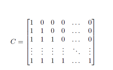
Each element in \(C\) has a value of 1 or 0.

• If \(C_{ij} = 1\) this means that at timestep \(i\) the model can observe the value at timestep \(j\) when predicting timestep \(i + 1\)

Feed Forward Network

• This is a simple two-layer neural network with layer normalization

class FeedForward(nn.Module):
    def __init__(self, config: DecoderConfig):
        self.linear_1 = nn.Linear(config.embed_dim, config.get_intermediate_dim())
        self.linear_2 = nn.Linear(config.get_intermediate_dim(), config.embed_dim)
        self.dropout = nn.Dropout(config.ff_dropout_prob)
        self.activation = NewGELU()

    def forward(self, x):
        x = self.dropout(self.linear_2(self.activation(self.linear_1(x))))
        return x

Decoder Block

• Now that we have all the components of the decoder, we can just stack them up to get one decoder block as follows

class DecoderBlock(nn.Module):
    def __init__(self, config: DecoderConfig):
        super().__init__()
        self.config = config
        self.layer_norm_1 = nn.LayerNorm(config.embed_dim)
        self.layer_norm_2 = nn.LayerNorm(config.embed_dim)
        self.attention = MultiHeadSelfAttention(config)
        self.ffn = FeedForward(config)

    def forward(self, x, mask=None):
        x = x + self.attention(self.layer_norm_1(x), mask)
        x = x + self.ffn(self.layer_norm_2(x))

        return x

Decoder

• Now that we have the decoder block ready, we replicate it 12 times just like what is done in the GPT2 paper and put all the components in one forward pass

class PDPDecoderTransformer(nn.Module):
    def __init__(
        self,
        config: DecoderConfig,
    ):
        # transforms each bin into a vector of size config.d_model
        # and adds positional embeddings
        self.data_embeddings = DataEmbeddings(config)
        # decoder blocks
        decoder_block = DecoderBlock(config)
        self.decoder_blocks = _clones(decoder_block, config.num_decoder_layers)
        self.dropout = nn.Dropout(config.ff_dropout_prob)
        self.layer_norm = nn.LayerNorm(config.embed_dim)
        self.head = nn.Linear(config.embed_dim, config.num_of_bins)

    def forward(
        self,
        x: torch.Tensor,
        mask: torch.Tensor,
    ):
        B = x.size(0)
        pos = torch.arange(0, MAX_TIMESTEPS, device=x.device).long().unsqueeze(0).repeat(B, 1)
        x = self.data_embeddings(x, pos)
        for i, decoder_block in enumerate(self.decoder_blocks):
            x = decoder_block(x, mask)
        x = self.layer_norm(x)
        head_output = self.head(x)
        head_output = F.softmax(head_output, dim=-1)

        return head_output

Loss Functions

Cross Entropy Loss

• Cross entropy is the loss function used in most classification problems, it has a formula of :

  \( L(y, p) = -1 \frac{1}{n} \sum_{i = 1}^n \sum_{c = 1}^C y_{ij} \log (p_{ij}) \)

• We wanted to guide the model that some bins were more similar to each other, e.g. if the correct bin is 5 and you predict bin 10, you should have a higher loss than somebody who predicted bin 6.

  • So we are proposing different loss functions

Gaussian Cross Entropy Loss

• This is very similar to cross entropy but with a slight modification. \(y\) is now a gaussian centered around the index of the correct bin, instead of a one-hot vector.
• The formula is still
  \( L(y, p) = -1 \frac{1}{n} \sum_{i = 1}^n \sum_{c = 1}^C y_{ij} \log (p_{ij}) \)
  but \(y\) represents a different vector.

STD_DEV = 0.27
# config.num_of_bins = 10
gaussians = torch.zeros(config.num_of_bins, config.num_of_bins, device=device)
x = torch.arange(config.num_of_bins, device=device)
for mean_around in range(config.num_of_bins):
    g_x = torch.exp(-((x - mean_around) ** 2) / (2 * STD_DEV ** 2))
    g_x = g_x / torch.sum(g_x)
    gaussians[mean_around] = g_x
# you can then access the gaussian vector through indexing the tensor
print(gaussians[4])
# tensor([0.0000e+00, 1.5516e-27, 1.2142e-12, 1.0481e-03, 9.9790e-01, 1.0481e-03, 1.2142e-12, 1.5516e-27, 0.0000e+00, 0.0000e+00])

• This way the model understands that it should have a lower loss if the bin predicted is close to the correct bin, instead of just treating close predictions the same as predictions far from the correct bin.

Custom Ordinal Cross Entropy Loss

• This adds a factor that also penalizes the model more if the bin is farther from the correct index.

• It has a formula of

  \( L(y, p) = -1 \frac{1}{n} \sum_{i = 1}^n (idx_{predicted} - idx_{correct})^2 \sum_{c = 1}^C y_{ij} \log (p_{ij}) \)

After trying all of these approaches, they provided similar results, so we went with the regular cross entropy.

Inference

Predict Max Bin

• This was the naive approach that we decided on earlier in the experiment, we would pick the bin that had the highest probability of being correct.

Weighted Average

In this method, we need to define two arrays

• pred : shape (1, # bins) for a single example, which we will refer to
  as p where \( p_i = p(y = bin_i) \)
• bin representation values: shape (1, # bins), which we will refer to
  as r, where \(r_i\) is the value we use to represent \(bin_i\)

We take the weighted average of the representation value of the top k bins, where the weights are the probabilities of each of the top k bins

e.g. if \( r = [100, 500, 1000, 2000, 5000], p = [0.25, 0.45, 0.15, 0.1, 0.05] \) and k = 2
our prediction would be \( y = \frac{p2∗r2+p1∗r1}{p1+p2} = \frac{0.45∗500+0.25∗100}{0.45+0.25} = 357.14 \)

But we added a condition before doing this, we will take the top k bins or
until the sum of the first n bins reaches 50%
e.g. if k = 3 and \(p = [0.25, 0.45, 0.15, 0.1, 0.05]\), we would only take bins 1 and 2, as \( p1 + p2 > 0.5 \)
You can tune the percentage that you stop before depending on your problem.

The second approach was much better than the first one especially in the later month as the model error accumulates and the model is less sure of its predictions

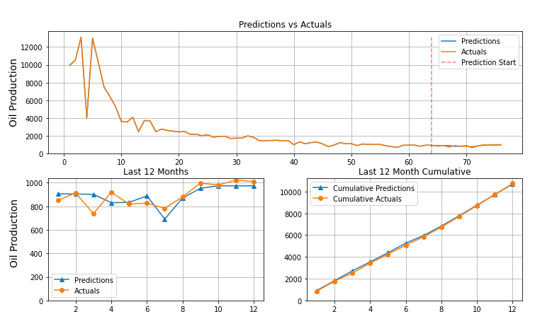
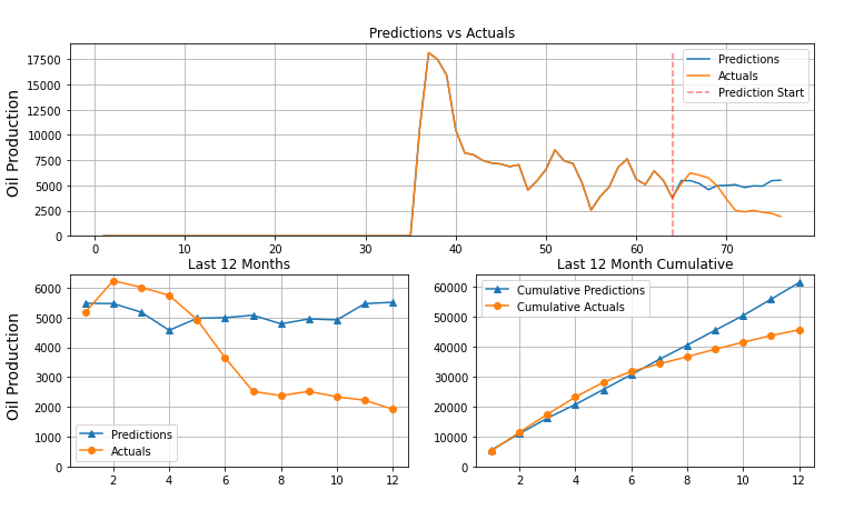
Results

• The model's performance was indicative of actual learning and sucessful training but it did has not outperformed the current model at Raisa.

  

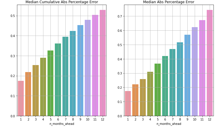
• Here are some examples of model predictions.

  

  

  

  

Conclusion

• During our experiment, we used the transformer in a different domain in which it is usually used.
• We found out that with a lot of tweaks the model shows signs of learning, but it still doesn't outperform the current model at Raisa
• The upside of this is that it is easier to scale up the transformer, we plan on experimenting with multivariate classification.
  • We would make the model predict the oil and gas data simultaneously and make use of both features.
• This experiment could give the transformer the edge it needs in order to surpass the performance of the current model.

References and Resources

• Language Models are Unsupervised Multitask Learners - The original GPT2 paper
• The Illustrated Transformer - Visual Explaination for the transformer
• minGPT - Code implementation for GPT2 by Andrej Karpathy
• The Annotated GPT2 - Visual Explanation for GPT2